sparse auto-encoders

Dec 31, 2024

Sparse auto-encoders are getting more popular. This is coupled with the emergence of tools to visualize deep neural networks like openai’s microscope (which is now shutdown apparently) and a new llm interperability project (the original repo of which has been taken down, link is a fork). These projects leveraged sparse auto-encoders, in part, to gain insight into why deep artificial neural networks make decisions the way they do. There seems to be something interesting to the idea because they keep deleting the projects, so I thought I would look into what it is, and see if I can make a simple example of a sparse auto encoder.

Sparse Auto-Encoders

What are sparse auto encoders? First let’s discuss what auto encoders are generally. Auto encoders are a type of neural network that is attempting to recreate it’s input. This is different from say an artificial neural network that is attempting predict some target value that is different from the input values. Here is an example of an auto encoder in pytorch:

import torch
import torch.nn as nn

# Define the autoencoder class
class SparseAutoencoder(nn.Module):
    def __init__(self):
        super(SparseAutoencoder, self).__init__()
        self.encoder = nn.Sequential(
            nn.Linear(28 * 28, 128),
            nn.ReLU(),
        )
        self.decoder = nn.Sequential(
            nn.Linear(128, 28 * 28),
            nn.Sigmoid(),  # Output in range [0, 1]
        )

    def forward(self, x):
        encoded = self.encoder(x)
        decoded = self.decoder(encoded)
        return encoded, decoded

We have two parts to the model:

An encoder that creates a smaller representation of the input
A decoder that expands that compressed representation back out into full size

Through the weights and biases of the artificial neural network, we attempt to create a model that can recreate values from the input class. The example we will use later is to recreate image from the mnist dataset, a dataset of handwritten numbers. We will attempt to train a neural network that can recreate the image of the written number.

Sparsity is a concept in machine learning to attempt to approximate a large matrix using a smaller one. We use this in neural networks to create smaller groups of activating neurons that approximage larger groups. I.e. if our full model would normally require 100 neurons activating to get somethig correct, we attempt to learn the same decision boundry with only 20 neurons activating. This “sparse” representation enables us to have more compact models that we can reason about more easily, with the potential trade off of model prediction quality.

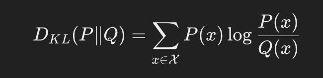
To do this, we add to the loss function a component that penalizes more neurons activating within hidden layers. There are a few good functions to do this, but the one we will use is Kullback–Leibler divergence (kl divergence). The formula is used in general to quantify the difference between two distributions. Here we see the general formula for a discrete distribution where P is our target distribution and Q is our actual distribution.

For sparse autoencoders, we can make use of this by having the target distribution be the percentage of neurons we wish to be active, and then actual distribution be the sum of the model’s hidden layer neurons actually activating. Thankfully, this is a discrete distribution with only two values, neuronn on (p = 1) and off (p = 0), and so we can decompose this quite nicely:

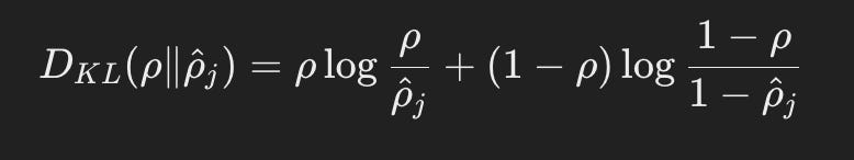
Just to solidify understanding, our formula has two parts which encapsulates all the discrete possibilities of the distribution. We compare the percentage of hidden neurons that are activated with our target activation percentage, and the percentage that aren’t activated with the inverse of our activation percentage. We then add those together to get our kl divergece value. Here we can see this equivalently in code:

# Sparse penalty (KL divergence)
def kl_divergence(p, q):
    return p * torch.log(p / q) +
           (1 - p) * torch.log((1 - p) / (1 - q))

And now we can put this together with a training loop to see how well our auto encoder performs. The main call out in this code is our two hyper parameters, our target activation distribution (which we set to 0.05, i.e. 5% of neurons activating) and our beta value which signifies how penalize the model should be for an activation that exceeds our target activation distribution (which we set to 0.1). Both of these are hyperparameters that one can play around with to get different results.

import torch
import torch.nn as nn
import torch.optim as optim
from torchvision import datasets, transforms
from torch.utils.data import DataLoader
import matplotlib.pyplot as plt

# Define the autoencoder class
class SparseAutoencoder(nn.Module):
    def __init__(self):
        super(SparseAutoencoder, self).__init__()
        self.encoder = nn.Sequential(
            nn.Linear(28 * 28, 128),
            nn.ReLU(),
        )
        self.decoder = nn.Sequential(
            nn.Linear(128, 28 * 28),
            nn.Sigmoid(),  # Output in range [0, 1]
        )

    def forward(self, x):
        encoded = self.encoder(x)
        decoded = self.decoder(encoded)
        return encoded, decoded

# Sparse penalty (KL divergence)
def kl_divergence(hidden_layer_output):
    mean_activation = torch.mean(hidden_layer_output, dim=0)
    kl_divergence = torch.sum(
        sparsity_level * torch.log(sparsity_level / (mean_activation + 1e-5)) +
         (1 - mean_activation) * torch.log((1 - sparsity_level) / (1 - mean_activation + 1e-5))
    )
    return kl_divergence

def loss(y_true, y_pred, encoded):
  loss = criterion(y_pred, y_true)
  sparsity_loss = kl_divergence(encoded)
  return loss + beta * sparsity_loss

# Load MNIST dataset
transform = transforms.Compose([
    transforms.ToTensor(),
])

train_dataset = datasets.MNIST(root="./data", train=True, transform=transform, download=True)
train_loader = DataLoader(train_dataset, batch_size=64, shuffle=True)

device = torch.device("cuda" if torch.cuda.is_available() else "cpu")

# Initialize model, loss function, and optimizer
model = SparseAutoencoder().to(device)
criterion = nn.MSELoss()
optimizer = optim.Adam(model.parameters(), lr=0.001)

# Training loop
epochs = 20
sparsity_target = 0.05
beta = 0.1  # Weight of sparsity penalty

for epoch in range(epochs):
    model.train()
    epoch_loss = 0
    for images, _ in train_loader:
        images = images.view(-1, 28 * 28).to(device)

        # Forward pass
        encoded, decoded = model(images)

        total_loss = loss(images, decoded, encoded)

        # Backward pass
        optimizer.zero_grad()
        total_loss.backward()
        optimizer.step()

        epoch_loss += total_loss.item()

    print(f"Epoch [{epoch + 1}/{epochs}], Average Loss: {epoch_loss / len(train_loader):.4f}")


# Visualize original and reconstructed images
def visualize_reconstruction(model, data_loader):
    model.eval()
    with torch.no_grad():
        images, _ = next(iter(data_loader))
        images = images.view(-1, 28 * 28).to(device)
        _, decoded = model(images)

        # Plot original and reconstructed images
        images = images.cpu().view(-1, 1, 28, 28)
        decoded = decoded.cpu().view(-1, 1, 28, 28)

        fig, axes = plt.subplots(2, 10, figsize=(10, 2))
        for i in range(10):
            axes[0, i].imshow(images[i].squeeze(), cmap="gray")
            axes[0, i].axis("off")
            axes[1, i].imshow(decoded[i].squeeze(), cmap="gray")
            axes[1, i].axis("off")
        plt.show()

visualize_reconstruction(model, train_loader)

and then here is our training output

Epoch [1/20], Average Loss: 0.1116
Epoch [2/20], Average Loss: 0.0772
Epoch [3/20], Average Loss: 0.0719
Epoch [4/20], Average Loss: 0.0701
Epoch [5/20], Average Loss: 0.0676
Epoch [6/20], Average Loss: 0.0654
Epoch [7/20], Average Loss: 0.0641
Epoch [8/20], Average Loss: 0.0631
Epoch [9/20], Average Loss: 0.0623
Epoch [10/20], Average Loss: 0.0621
Epoch [11/20], Average Loss: 0.0616
Epoch [12/20], Average Loss: 0.0602
Epoch [13/20], Average Loss: 0.0595
Epoch [14/20], Average Loss: 0.0578
Epoch [15/20], Average Loss: 0.0589
Epoch [16/20], Average Loss: 0.0563
Epoch [17/20], Average Loss: 0.0574
Epoch [18/20], Average Loss: 0.0566
Epoch [19/20], Average Loss: 0.0564
Epoch [20/20], Average Loss: 0.0564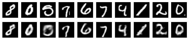

Our training output. Top is the true data, bototm is our estimation

Which I think is not too shabby. Close lines get a bit blurry, but overall not a bad job. Here we can also see our mean activations per neuron

model.eval()
all_encoded = []

# Collect encoded activations from the entire training set
with torch.no_grad():
    for images, _ in train_loader:
        images = images.view(-1, 28 * 28).to(device)
        encoded, _ = model(images)
        all_encoded.append(encoded)

# Stack all encoded activations
all_encoded = torch.cat(all_encoded, dim=0)

# Calculate the mean activation across all samples
mean_activation = torch.mean(all_encoded, dim=0).cpu().detach().numpy()

# Plot the mean activation of the hidden layer
plt.figure(figsize=(10, 6))
plt.plot(mean_activation, label="Mean Activation", color="blue")
plt.xlabel("Neuron Index")
plt.ylabel("Mean Activation")
plt.title("Mean Activation of Hidden Layer After Training")
plt.legend()
plt.grid(True)
plt.show()

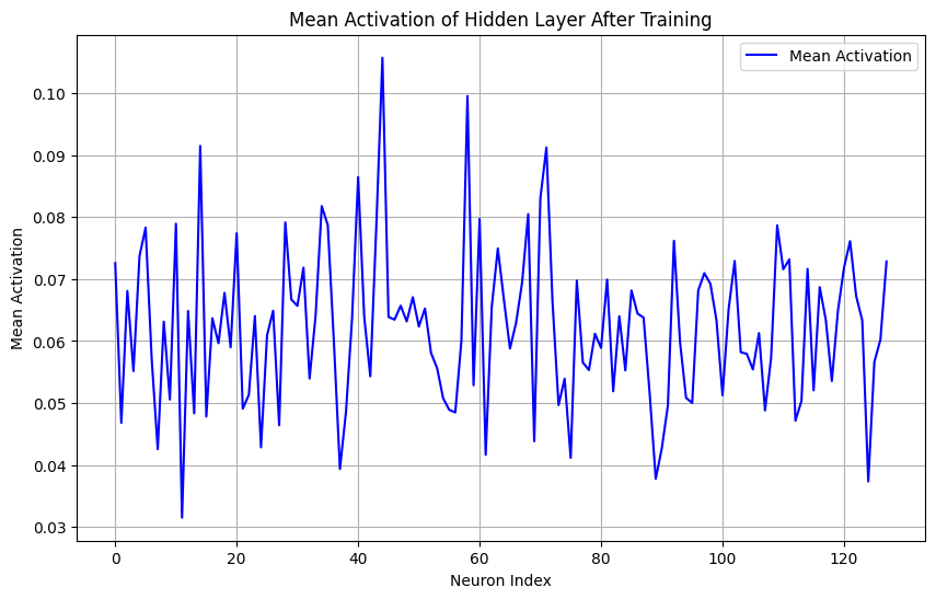
Which is nice evidence that our neurons are only activing around 6% or 7% of the time, which is roughly around our target.

Thus, we have a model network that is much easier to analyze since only a small subset of neurons our activating. The goal would the be to attempt to understand what these neuron activations represent, either as individual neurons or as groups called circuits. This is a growing field called mechanistic interpretability.

Conclusion

Why do we do this? Because neural networks are difficult to understand, but there growing importance in our lives means it’s more important to understand them. Breaking them down into smaller parts allows us to better understand them.

From openai’s circuit project, which used it’s microscope web app, we can see the two ideas we care about. Feautre visualization which is visualizing what in particular a network is looking for, and attribution which works backwards to understand what part of the network contributes to the end decision.

We can use sparse auto encoders to achieve these goals. A good example of this is the llama 3 interpretability project, which uses sparse auto encoders injected into llms to turn dense representations into sparse representations which are easier to analyze because they are more discrete.

It would then be up to us to figure out what these features represent. From the circuits project linnked above, we see a visualization of features in an image detection neural network. While we may have an intuition into roughly what it’s detecting, it’s difficult to know exactly what it is.

Overall there is a lot of cool work occuring in this space, and we nice to learn about how these are being used to understand more complex neural networks like multi billion parameter LLMs.

Important Works

Discussion about this post