phi-flow

I’m currently reading through physics based deep learning, and there are a lot of really wonderful ideas to write about. I’m going to strive for one a chapter. For the first chapter, they introduce a really cool python package called PhiFlow. I wanted to take a moment to showcase what PhiFlow is, and walkthrough in detail the example provided.

PhiFlow

Phiflow is a python package that makes it easier to use deep learning models for physics simulations by solving partial differential equations. It does so by creating and abstracting the actual model function that is being optimized against. For example, if we are simulating a fluid via a partial differential equation, it provides handy tools to create the fields, create the partial differential function, and then hook tthese into any of the deep learning packages. Lastly, it integrates well with charting libraries for visualizations.

Physics Simulation

Let’s start by explaining the fluid simulation example to simulate a smoke plume. We start by importing phyflow

from phi.flow import *

Next, we create the grid where the simulation will occur. We can think of this as pixels on a screen, where each pixel represents the unit cell with which we will sample our simulation. We do so in 2d for ease of simulation. Here we are using two different methods for sampling. In the first, we use a CenteredGrid where each cell is represented by the average within that cell via the center. We use this to represent the density of smoke. The second is a StaggeredGrid where each cell is represented via the values at the cell’s edges. We use this to represent velocity. We prefer to use a StaggeredGrid with velocity because we want to map the total outflow of a cell in both the x and y direction, something we can’t do from a single number. The other point to bring up is the extrapolation boundry. Since we are simulating motion, we can make a decision of how far outside our simulation boundry we wish to simulate for continuity. The decision for which to select comes down to what values must be stored for the simulation to be accurate.

smoke = CenteredGrid(0, extrapolation.BOUNDARY, x=32, y=40, bounds=Box(x=32, y=40))  # sampled at cell centers
velocity = StaggeredGrid(0, extrapolation.ZERO, x=32, y=40, bounds=Box(x=32, y=40))  # sampled in staggered form at face centers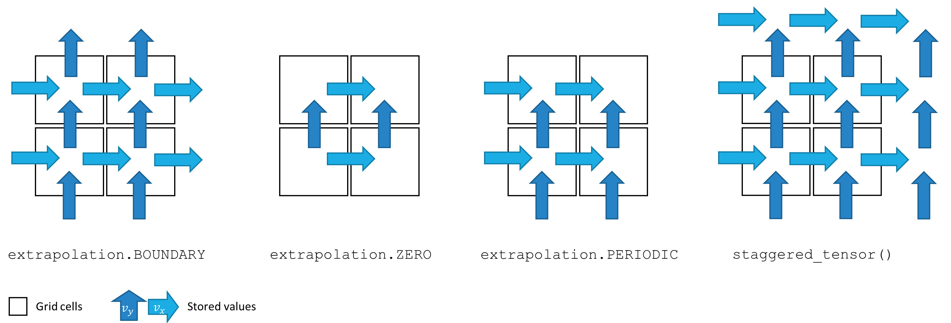

For our fluid, we now need something to represent where the inflow of the fluid will come from. You can think of this as the “input” to the system we are creating. We will represent this as a tensor at 4 different locations on the Cartesian grid, and will then mark a section of the grid at those locations as smoke for each inflow. Tensors are used as an abstraction over any n dimensional data object. Here we essentially just use it as an array.

INFLOW_LOCATION = tensor([(4, 5), (8, 5), (12, 5), (16, 5)], batch('inflow_loc'), channel(vector='x,y'))
INFLOW = 0.6 * CenteredGrid(Sphere(center=INFLOW_LOCATION, radius=3), extrapolation.BOUNDARY, x=32, y=40, bounds=Box(x=32, y=40))

Now let’s add these inflows into our smoke grid. We can use phi-flows handy shorthand for plotting here as well to see the inflows visually.

smoke += INFLOW
vis.plot(smoke)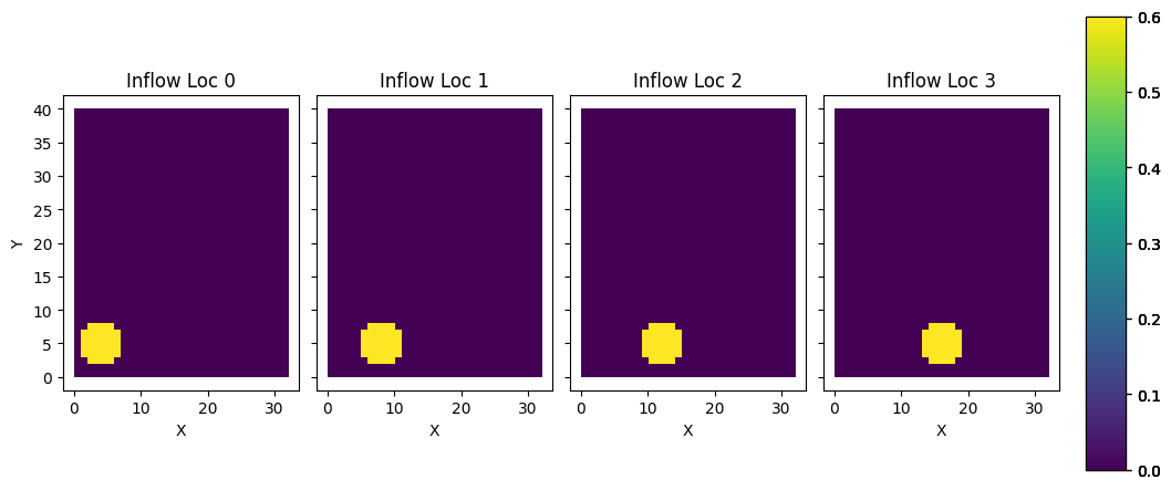

The starting groups of smoke for our simulation. Each one will have a seperate simulation run.

Now let’s calculate the buoyancy force of the fluid. One generally thinks of buoyancy force whenever we see an object in water. The object floats because the water pushes up on the object more than the object pushes down on the water. This force from the fluid is called the buoyancy force. In the context of our simulation, the smoke is in air, and thus the smoke being less dense then the air is pushing up on on the air the same way water pushes up on a floating object. We represent this with a force with a vertical vector (0, 0.5). If we were running this on a real gas, we would get this force from empircal study.

We base the amount of force off of the amount of smoke at each pixel, and update the velocity values at each edge to correspond with this. Here we are using the matmul symbol `@` to map between the center based values of the smoke to the staggered values of the velocities. Normally the matmul symbol is used for matrix muliplication, but for these field objects we override that operator with this translation operation. This forms the basis of our starting force.

buoyancy_force = smoke * (0, 0.5) @ velocity
vis.plot(buoyancy_force)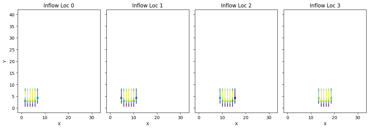

We also need to calculate the velocities of the smoke from the inflow point. We are essentially telling each unit cell which direction smoke should move once entered into the system, given the starting location of the smoke. We do so by first adding our starting velocities to the velocity grid, and then running the make_incompressible helper function. Why is it called make incompressible? It is because our fluid here is a gas. Fluids like water are already compressed when allowed to come to rest, while gases are not. This creates a difference in the way they move, which needs to be reflected in the simulation. This also makes big difference in the way that calculations are propogated.

velocity += buoyancy_force
velocity, _ = fluid.make_incompressible(velocity)
vis.plot(velocity)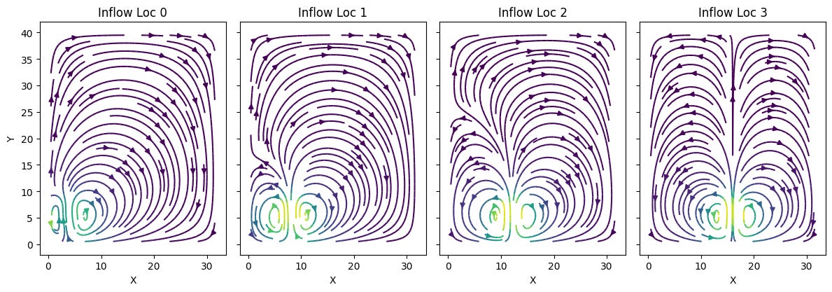

We can now go ahead and run the entire simulation by repeating these steps multiple times. I won’t dive too deep into the math behind the next few lines of code, but essentially all it is doing is taking the previous values, generating a solution to the incompressible navier-strokes equation, and then applying it to our grid for 20 timesteps.

trajectory = [smoke]
velocities = [velocity]
for i in range(20):
  print(i, end=' ')
  smoke = advect.mac_cormack(smoke, velocity, dt=1) + INFLOW
  buoyancy_force = smoke * (0, 0.5) @ velocity
  velocity = advect.semi_lagrangian(velocity, velocity, dt=1) + buoyancy_force
  velocity, _ = fluid.make_incompressible(velocity)
  trajectory.append(smoke)
  velocities.append(velocity)

trajectory = field.stack(trajectory, batch('time'))
vis.plot(trajectory, animate='time')

velocities = field.stack(velocities, batch('time'))
vis.plot(velocities, animate='time')

Adding Some Learning

Let’s look at how we can set this up to be trained on a neural network!

Let’s start by importing the pytorch handler

from phi.torch.flow import *

and setup the simulation as before

INFLOW_LOCATION = tensor([(4, 5), (8, 5), (12, 5), (16, 5)], batch('inflow_loc'), channel(vector='x,y'))
INFLOW = 0.6 * CenteredGrid(Sphere(center=INFLOW_LOCATION, radius=3), extrapolation.BOUNDARY, x=32, y=40, bounds=Box(x=32, y=40))
initial_smoke = CenteredGrid(0, extrapolation.BOUNDARY, x=32, y=40, bounds=Box(x=32, y=40))
initial_velocity = StaggeredGrid(math.zeros(batch(inflow_loc=4)), extrapolation.ZERO, x=32, y=40, bounds=Box(x=32, y=40))

However we make a significant change to our simulation timestep function by adding in the loss calculation component. Here we are using the mean squared error between where the smoke should be and where the neural network believes it should be.

def simulate(smoke: CenteredGrid, velocity: StaggeredGrid):
  for _ in range(20):
    smoke = advect.mac_cormack(smoke, velocity, dt=1) + INFLOW
    buoyancy_force = smoke * (0, 0.5) @ velocity
    velocity = advect.semi_lagrangian(velocity, velocity, dt=1) + buoyancy_force
    velocity, _ = fluid.make_incompressible(velocity)
  loss = math.sum(field.l2_loss(diffuse.explicit(smoke - field.stop_gradient(smoke.inflow_loc[-1]), 1, 1, 10)))
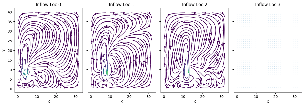
  return loss, smoke, velocity

We use this function to get a mapping of the initial gradients. This is essentially the model that is being trained, as we use this set of gradients to determine the next step in our simulation. The loss is used internally to help update weights, while the velocities are used as an input in the next times step after being adjusted. Our smoke is the loss, and the velocities are updated via back propogation in response to that loss.

Here we can see the initial gradients of the model:

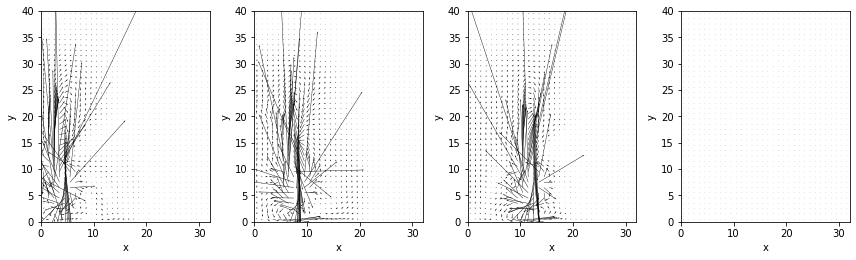
And some of the velocities predicted initially from those gradients:

Model attempting to learn the velocities. Not sure what happened with loc 3.

From there we run the learning step like we would for any other machine learning training. We could then plug this loss into a machine learning model for training specific weights. Here I am keeping the intermediary steps as well just to visualize.

sim_grad = field.gradient(simulate, wrt='velocity', get_output=True)
sim_trajectory = [initial_smoke]

for opt_step in range(4):
  (loss, final_smoke, _v), velocity_grad = sim_grad(initial_smoke, initial_velocity)
  print(f"Step {opt_step}, loss: {loss}")
  initial_velocity -= 0.01 * velocity_grad
  sim_trajectory.append(final_smoke)

sim_trajectory = field.stack(sim_trajectory, batch('time'))
vis.plot(sim_trajectory, animate='time')

Running this still took a great deal of computing. What this is visualizing is essentially the model’s next step prediction given the gradients it has, which is why the visual is so stiff. By calculating the difference between the expectation and the gradient, we can calculate a loss function, which can be then plugged into a neural network to then update those gradients to be more accurate. Because we aren’t plugging into a model, these don’t get any better.

Conclusion

This project is an exciting example of the very early world that is utilizing machine learning models for physics simulation. I’m really excited to see what this technology can do for the physics that is more difficult to simulate via traditional means. Instead we can just setup that basis of a simulation, add in empirical data, and see what the model comes up with!