can recurrent neural networks solve fluids?
In the last post, I managed to finally get the simulation data to work with an auto encoder model. However, the models actual output was very poor. Today, I’ll start exploring machine learning models specifically tailored to handle data that is both spatial and temporal or spatiotemporal, starting with Recurrent Neural Networks. As a reminder, we will be testing this against our simulated fluid of gas. Here is the video, which you can find code for in the previous blog post:
Recurrent Neural Networks
Recurrent Neural Networks (RNNs) is an order dependent type of neural network where each output in the sequence gets fed back into the model for the next input. In the context of time series data, we feed each time t of the series into the model to get an output. Then we condition our next input (t + 1) on that output to get the next output. We repeat this for every time step we wish. Thus we take into consideration the previous output times output when considering the current output.
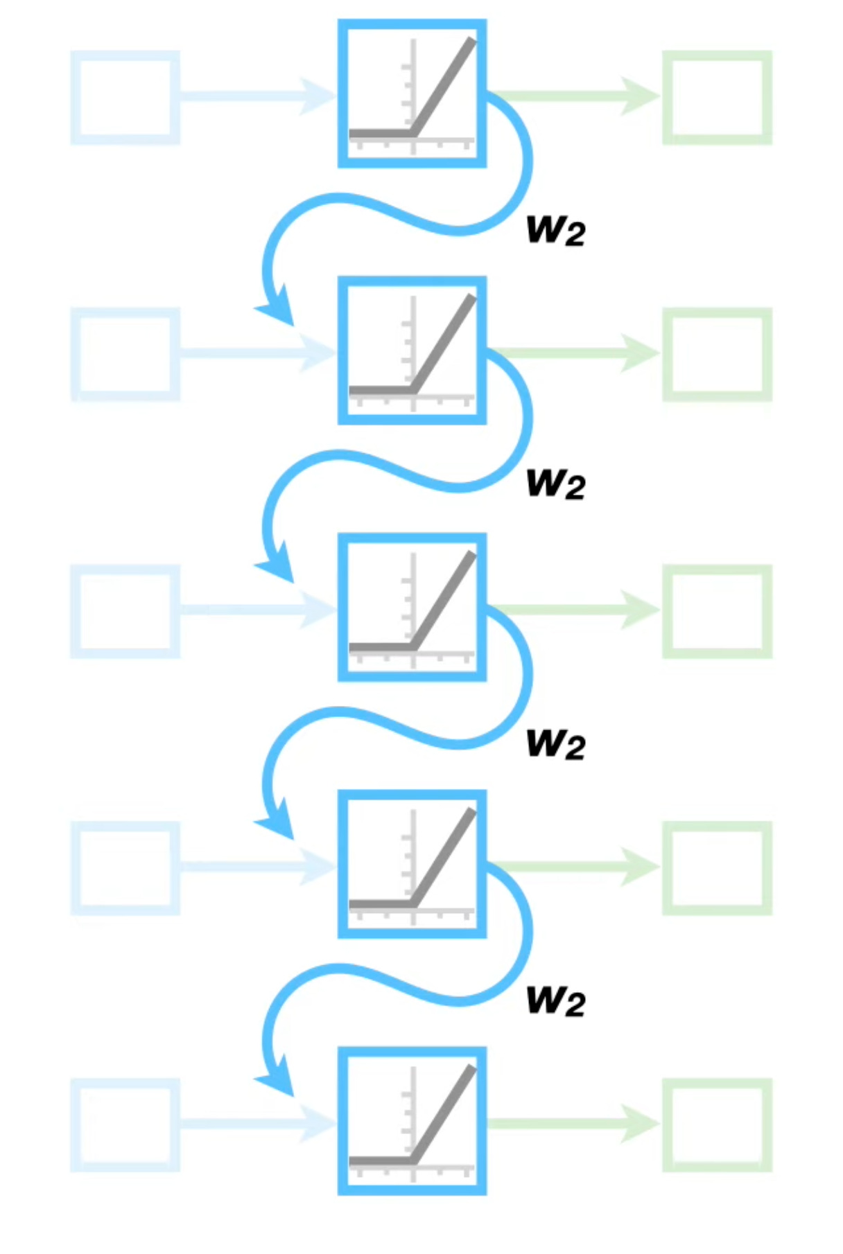
Recurrent Neural Networks tend to suffer in a few key ways
The models don’t store information for a long time. If we increase the number of steps, previous steps a long time ago that may be important now aren’t weighted more heavily.
The model can take a while for training and inference if the number of steps is large.
The models suffer from exploding an vanishing gradients. Multiplying large weights many times causes them to grow exponentially, while multiplying small ones makes them close to zero. Both are undesired local minima.
This is why a simple RNN tends to not be used in practice.
A fix is Long Short Term Memory (LSTM) models. These models enhance the RNN by including memory units that allow data to be saved while the model runs. We can then update our long and short term memory rather than the output directly. This gets us around at least problems one and two above.
The way we update our model is a series of gates. These are the input gate, the output gate, and the forget gate. The forget gate determines how much of the long term memory we should forget, the input gate determine how much we should update the long term memory with new information, and the output gate determines how much of the short term memory (the previous output) should be considered in the final output.
Let’s look at a visual of this, followed by an explanation.
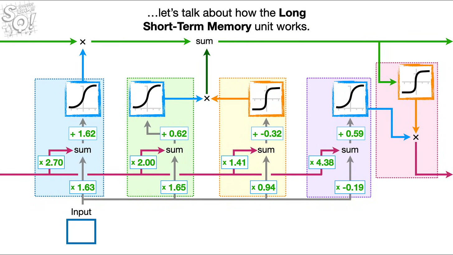
We see the long term memory represented by the green line on top affected by our blue forget gate on the left, and the input gate consisting of the green and yellow gates in the center. We then have our short term memory represented by the red line on bottom, going into our output gate represented by the purple and red on the right. With these combinations of gates, we are able to keep information over longer periods while also avoiding the gradients from exploding or disappearing.
I won’t dive into the math here, but it’s a series of matrix multiplications & additions followed by activation functions. If you are interested in a visual explanation you can watch the statquest video linked on the image above, or the code below will lay out all the actual operations.
Let’s look at a simple coding example using an LSTM to predict a sin wave.
We will Start by generating some random data points to learn along a sin wave.
# Sine Wave Data Generator
def generate_sine_data(seq_len=50, num_samples=1000):
    x = np.linspace(0, 100, num_samples)
    y = np.sin(x)
    X, Y = [], []
    for i in range(len(y) - seq_len):
        X.append(y[i:i+seq_len])
        Y.append(y[i+seq_len])
    X = torch.tensor(X, dtype=torch.float32).unsqueeze(-1)  # (batch, seq_len, 1)
    Y = torch.tensor(Y, dtype=torch.float32).unsqueeze(-1)  # (batch, 1)
    return X, Y
We’ll have two big parts of our LSTM. The outer layer will feed our previous values output into our LSTM unit. Our unit will do the actual calculation to turn our input into the output using the various gates discussed above.
Let’s start with the outer feeding function. We’ll initialize our long and short term memory. Then we will query our LSTM cell for the next output, updating our memory as we go. We’ll finish by decoding the prediction from our LSTM, and return the predicted value.
def forward(self, x):
        batch_size, seq_len, _ = x.size()
        short_term_memory = torch.zeros(batch_size, self.hidden_size, device=x.device)
        long_term_memory = torch.zeros(batch_size, self.hidden_size, device=x.device)

        for t in range(seq_len):
            input_t = x[:, t, :]
            short_term_memory, long_term_memory = self.lstm_cell(input_t, short_term_memory, long_term_memory)

        output = self.fc(short_term_memory)
        return output
Now let’s look at the actual cell itself. We’ll start by calculating how much our input and short term memory should affect our long term memory. We’ll pass this value through all of our gates, and then update the long term memory with the results. We’ll finish by passing our output gate results with the long term memory. This is just a coded representation of the previous photo.
def forward(self, input_t, short_term_memory_prev, long_term_memory_prev):
        # Calculate gates and candidate memory
        combined = self.x2h(input_t) + self.h2h(short_term_memory_prev)
        input_gate, forget_gate, candidate_memory, output_gate = combined.chunk(4, dim=1)

        # Apply activations
        input_gate = torch.sigmoid(input_gate)
        forget_gate = torch.sigmoid(forget_gate)
        candidate_memory = torch.tanh(candidate_memory)
        output_gate = torch.sigmoid(output_gate)

        # Update long-term and short-term memory
        long_term_memory = (forget_gate * long_term_memory_prev) + (input_gate * candidate_memory)
        short_term_memory = output_gate * torch.tanh(long_term_memory)

        return short_term_memory, long_term_memory
And now, the entire training process:
import torch
import torch.nn as nn
import torch.optim as optim
import numpy as np
import matplotlib.pyplot as plt

# LSTM Cell Implementation
class LSTMCell(nn.Module):
    def __init__(self, input_size, hidden_size):
        super(LSTMCell, self).__init__()
        self.input_size = input_size
        self.hidden_size = hidden_size
        self.x2h = nn.Linear(input_size, 4 * hidden_size)
        self.h2h = nn.Linear(hidden_size, 4 * hidden_size)

    def forward(self, x_t, h_prev, c_prev):
        gates = self.x2h(x_t) + self.h2h(h_prev)
        i_t, f_t, g_t, o_t = gates.chunk(4, dim=1)

        i_t = torch.sigmoid(i_t)
        f_t = torch.sigmoid(f_t)
        g_t = torch.tanh(g_t)
        o_t = torch.sigmoid(o_t)

        c_t = f_t * c_prev + i_t * g_t
        h_t = o_t * torch.tanh(c_t)

        return h_t, c_t

# LSTM Model chaining the cell over time
class CustomLSTM(nn.Module):
    def __init__(self, input_size, hidden_size, output_size=1):
        super(CustomLSTM, self).__init__()
        self.hidden_size = hidden_size
        self.lstm_cell = LSTMCell(input_size, hidden_size)
        self.fc = nn.Linear(hidden_size, output_size)

    def forward(self, x):
        batch_size, seq_len, _ = x.size()
        h_t = torch.zeros(batch_size, self.hidden_size, device=x.device)
        c_t = torch.zeros(batch_size, self.hidden_size, device=x.device)

        for t in range(seq_len):
            x_t = x[:, t, :]
            h_t, c_t = self.lstm_cell(x_t, h_t, c_t)

        output = self.fc(h_t)
        return output

# Sine Wave Data Generator
def generate_sine_data(seq_len=50, num_samples=1000):
    x = np.linspace(0, 100, num_samples)
    y = np.sin(x)
    X, Y = [], []
    for i in range(len(y) - seq_len):
        X.append(y[i:i+seq_len])
        Y.append(y[i+seq_len])
    X = torch.tensor(X, dtype=torch.float32).unsqueeze(-1)  # (batch, seq_len, 1)
    Y = torch.tensor(Y, dtype=torch.float32).unsqueeze(-1)  # (batch, 1)
    return X, Y

# Setup
SEQ_LEN = 50
X, Y = generate_sine_data(seq_len=SEQ_LEN)
model = CustomLSTM(input_size=1, hidden_size=50)
criterion = nn.MSELoss()
optimizer = optim.Adam(model.parameters(), lr=0.01)

# Training loop
NUM_EPOCHS = 20
for epoch in range(NUM_EPOCHS):
    model.train()
    optimizer.zero_grad()
    output = model(X)
    loss = criterion(output, Y)
    loss.backward()
    optimizer.step()
    print(f"Epoch {epoch+1}/{NUM_EPOCHS}, Loss: {loss.item():.6f}")

# Prediction and plotting
model.eval()
with torch.no_grad():
    preds = model(X).squeeze().numpy()
    true_vals = Y.squeeze().numpy()

plt.figure(figsize=(12, 5))
plt.plot(true_vals, label="True", linewidth=2)
plt.plot(preds, label="Predicted", linestyle="--")
plt.legend()
plt.title("Custom LSTM Output on Sine Wave")
plt.xlabel("Sample")
plt.ylabel("Value")
plt.grid(True)
plt.show()
We see that our LSTM does a good job at predicting the current step with help from previous steps! Now let’s see if we can do the same for our fluid simulation. We need to make one more update before we do.
Convolutional LSTM
Our LSTM currently considers only the temporal data, but doesn’t do much with regard to spatial data. To fix this for the moment, we will add a convolution term to our LSTM. Let’s do a quick detour to explain convolutions.
Convolutions
For our purposes, a convolution is a small filter passed over data, multiplying elements pairwise and then summing their results. Imagine you were trying to identify whether an image was a cat. One idea might be to slide your finger along the image top to bottom, left to right looking for particular features of cats like whiskers, paws, or fur. This is exactly what a convolution does. It attempts to learn what whiskers are, then creates a matrix of where those whiskers are in the image once it sees it. We can then use that matrix as a map of where the whiskers are, using it to decide whether a cat is in the image or not.
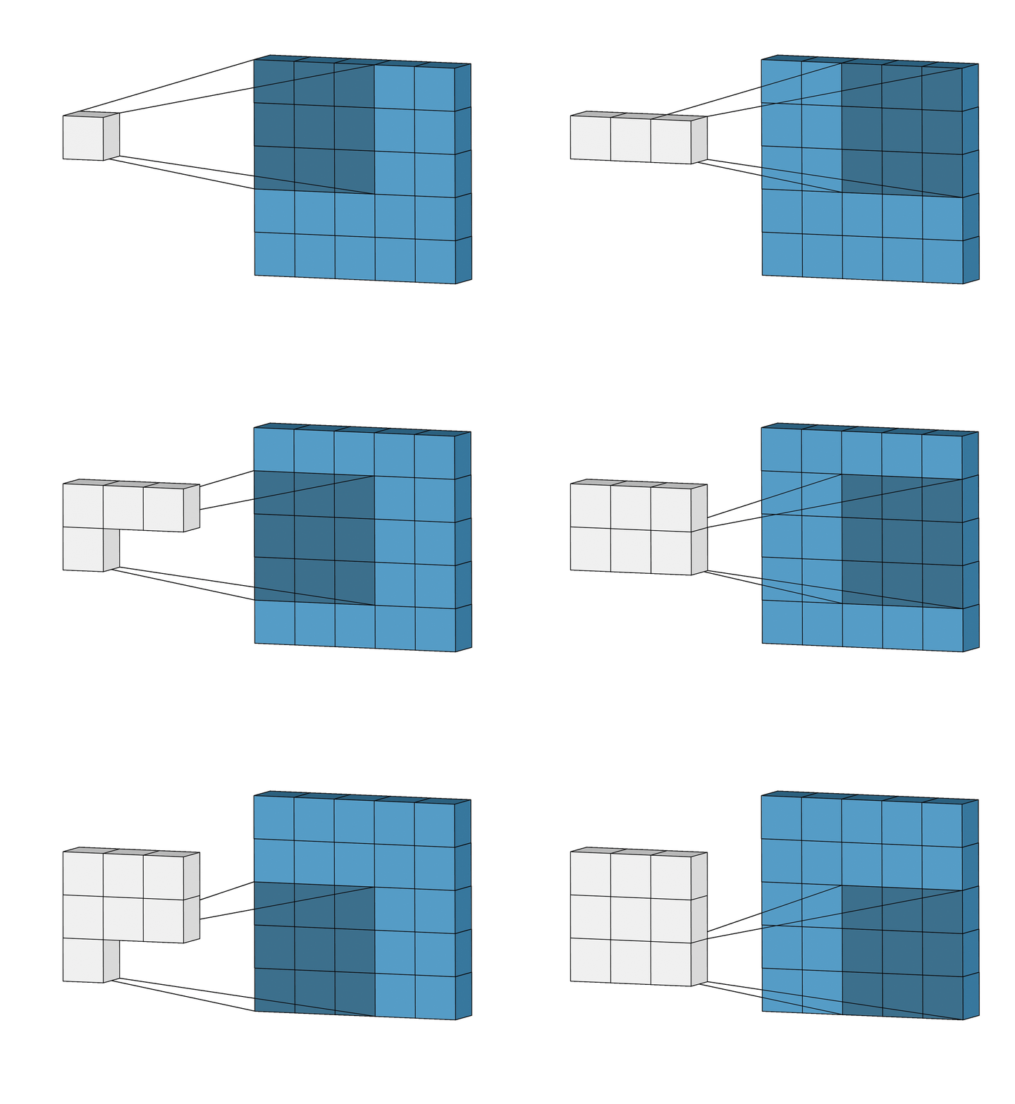
This is really great for fluids because fluids care about spatial features! We care about the density and velocity at one point to decide the density or velocity of the fluid at another point. As compared to linear evaluators, convolutions offer us an opportunity to extract these spatial features from the image data we have.
Let’s add convolutions to our fluid code.
Back to Fluids
Our cell code doesn’t change very much. The only real difference is that instead of linearly encoding our input, we use a convolution to encode the input.
def forward(self, x, short_term_memory, long_term_memory):
        # Combine input with short-term memory (previous hidden state)
        combined = torch.cat([x, short_term_memory], dim=1)
        conv_out = self.conv(combined)

        # Split the output into gates and cell candidate
        input_gate, forget_gate, output_gate, cell_candidate = torch.chunk(conv_out, 4, dim=1)

        # Apply activations for each gate
        input_gate = torch.sigmoid(input_gate)
        forget_gate = torch.sigmoid(forget_gate)
        output_gate = torch.sigmoid(output_gate)
        cell_candidate = torch.tanh(cell_candidate)

        # Update long-term memory (cell state)
        long_term_memory = forget_gate * long_term_memory + input_gate * cell_candidate

        # Update short-term memory (hidden state)
        short_term_memory = output_gate * torch.tanh(long_term_memory)

        return short_term_memory, long_term_memory
our outer layer changes a bit more, but not too much. Rather than our input being a single point, our input is now a sequence of steps in our simulation. So, the model must first catch up to the last point in the sequence, and then begin predicting the next set of steps in the simulation.
def forward(self, x_seq):
        # x_seq: (B, T, C, H, W)
        B, T, C, H, W = x_seq.size()
        short_term_memory = torch.zeros(B, self.convlstm.hidden_channels, H, W, device=x_seq.device)
        long_term_memory = torch.zeros(B, self.convlstm.hidden_channels, H, W, device=x_seq.device)

        # Process input sequence
        for t in range(T):
            x_t = self.encoder(x_seq[:, t])
            short_term_memory, long_term_memory = self.convlstm(x_t, short_term_memory, long_term_memory)

        # Predict future sequence
        predictions = []
        x_t = x_seq[:, -1]  # start with last input
        for _ in range(100):  # fixed 100-step rollout
            x_enc = self.encoder(x_t)
            short_term_memory, long_term_memory = self.convlstm(x_enc, short_term_memory, long_term_memory)
            x_t = self.decoder(short_term_memory)
            predictions.append(x_t.unsqueeze(1))

        return torch.cat(predictions, dim=1)  # (B, 100, C, H, W)
And now, the full training code + results:
import torch
import torch.nn as nn
import torch.optim as optim
from torch.utils.data import DataLoader, Dataset

# --- ConvLSTM Cell ---
class ConvLSTMCell(nn.Module):
    def __init__(self, input_channels, hidden_channels, kernel_size=3):
        super().__init__()
        padding = kernel_size // 2
        self.conv = nn.Conv2d(input_channels + hidden_channels, 4 * hidden_channels, kernel_size, padding=padding)
        self.hidden_channels = hidden_channels

    def forward(self, x, short_term_memory, long_term_memory):
        # Combine input with short-term memory (previous hidden state)
        combined = torch.cat([x, short_term_memory], dim=1)
        conv_out = self.conv(combined)

        # Split the output into gates and cell candidate
        input_gate, forget_gate, output_gate, cell_candidate = torch.chunk(conv_out, 4, dim=1)

        # Apply activations for each gate
        input_gate = torch.sigmoid(input_gate)
        forget_gate = torch.sigmoid(forget_gate)
        output_gate = torch.sigmoid(output_gate)
        cell_candidate = torch.tanh(cell_candidate)

        # Update long-term memory (cell state)
        long_term_memory = forget_gate * long_term_memory + input_gate * cell_candidate

        # Update short-term memory (hidden state)
        short_term_memory = output_gate * torch.tanh(long_term_memory)

        return short_term_memory, long_term_memory

# --- UNet + ConvLSTM Model ---
class ConvLSTMUNet(nn.Module):
    def __init__(self, input_channels=3, hidden_channels=32):
        super().__init__()

        self.encoder = nn.Sequential(
            nn.Conv2d(input_channels, 32, kernel_size=3, padding=1),
            nn.ReLU(),
            nn.Conv2d(32, 64, kernel_size=3, padding=1),
            nn.ReLU(),
        )

        self.convlstm = ConvLSTMCell(64, hidden_channels)

        self.decoder = nn.Sequential(
            nn.Conv2d(hidden_channels, 32, kernel_size=3, padding=1),
            nn.ReLU(),
            nn.Conv2d(32, input_channels, kernel_size=3, padding=1),
        )

    def forward(self, x_seq):
        # x_seq: (B, T, C, H, W)
        B, T, C, H, W = x_seq.size()
        short_term_memory = torch.zeros(B, self.convlstm.hidden_channels, H, W, device=x_seq.device)
        long_term_memory = torch.zeros(B, self.convlstm.hidden_channels, H, W, device=x_seq.device)

        # Process input sequence
        for t in range(T):
            x_t = self.encoder(x_seq[:, t])
            short_term_memory, long_term_memory = self.convlstm(x_t, short_term_memory, long_term_memory)

        # Predict future sequence
        predictions = []
        x_t = x_seq[:, -1]  # start with last input
        for _ in range(100):  # fixed 100-step rollout
            x_enc = self.encoder(x_t)
            short_term_memory, long_term_memory = self.convlstm(x_enc, short_term_memory, long_term_memory)
            x_t = self.decoder(short_term_memory)
            predictions.append(x_t.unsqueeze(1))

        return torch.cat(predictions, dim=1)  # (B, 100, C, H, W)

# --- Dataset for sequences ---
class FluidSequenceDataset(Dataset):
    def __init__(self, fluid_grids, history=3):
        self.history = history
        self.sequences = []
        for i in range(len(fluid_grids) - history):
            seq = []
            for j in range(history):
                g = fluid_grids[i + j]
                tensor = torch.stack([
                    torch.tensor(g.density, dtype=torch.float32),
                    torch.tensor(g.velocityx, dtype=torch.float32),
                    torch.tensor(g.velocityy, dtype=torch.float32)
                ], dim=0)
                seq.append(tensor)
            self.sequences.append(torch.stack(seq))

    def __len__(self):
        return len(self.sequences)

    def __getitem__(self, idx):
        return self.sequences[idx]

# --- Total Variation Loss for spatial smoothness ---
def total_variation(x):
    return torch.sum(torch.abs(x[:, :, :, :-1] - x[:, :, :, 1:])) + torch.sum(torch.abs(x[:, :, :-1, :] - x[:, :, 1:, :]))

# --- Training Loop ---
def train_model(model, dataloader, epochs=50, lr=0.001):
    optimizer = optim.Adam(model.parameters(), lr=lr)

    for epoch in range(epochs):
        total_loss = 0.0
        for seq_batch in dataloader:
            seq_batch = seq_batch.to(device)
            target = seq_batch[:, -1]  # supervise with next step

            optimizer.zero_grad()
            prediction = model(seq_batch)[:, 0]  # only predict one step for training

            loss = nn.functional.mse_loss(prediction, target)

            loss.backward()
            optimizer.step()
            total_loss += loss.item()

        print(f"Epoch {epoch+1}/{epochs}, Loss: {total_loss/len(dataloader):.6f}")

# --- Example Usage ---
if __name__ == "__main__":
    device = torch.device("cuda" if torch.cuda.is_available() else "cpu")
    model = ConvLSTMUNet().to(device)

    dataset = FluidSequenceDataset(fluid_grids, history=3)
    dataloader = DataLoader(dataset, batch_size=16, shuffle=True)

    train_model(model, dataloader, epochs=100, lr=0.001)

    # Predict 100 future timestamps and store in new array
    with torch.no_grad():
        sample_seq = dataset[0].unsqueeze(0).to(device)  # (1, T, C, H, W)
        future_predictions = model(sample_seq)  # (1, 100, C, H, W)
        print("Future prediction shape:", future_predictions.shape)

        # Extract density channel (index 0)
        future_densities = future_predictions[:, :, 0, :, :]  # (1, 100, H, W)
        print("Future density shape:", future_densities.shape)

    # `future_predictions` holds the 100-step rollout results
    # `future_densities` holds only the density values
It starts off really well, but appears to lose the plot as time goes on. A problem of only having roughly linear memory, and struggling to apply it as the gas disapates. Let’s see if we can improve this once again.
Self-Attention ConvLSTM
There are so many ways that transformers are brilliant. One of the simplest is that it solves the problem that our LSTMs have had so far: How do you manage memory over long periods of time without exploding or vanishing gradient? It does so via self-attention an idea I will briefly detour to before explaining how we can add a self attention memory module to our LSTM.
Self-Attention Detour
The way we have currently handled previous state has been focused on linearly passing the state forward at each iteration. The state at time t passes the memory along to state t+1. What would be nice though is if the state at t+1 was able to look at the entirety of the state before it rather than be forced to go through state t. This is exactly what self attention gets us.
Since it was discovered via natural language processing, I’ll use text generation as an example, and then shift back to fluids. I’ll also skip over the math for now, and explain some of it later. This example is stolen and abbreviated from the excellent 3blue1brown video.
Consider an example sentence like:
a fluffy blue creature roamed the verdant forest
In our existing LSTM example, we would have to pass a => fluffy => blue => … => forest. This means by the time we get to forest we may have lost the context of a fluffy blue creature. Even worse, our existing mechanism simply has memory, it doesn’t have an understanding as to what to do with that memory. We hope that the weights carry important information, but because we must pass through so many layers there is no guarantee that is the case.
With self-attention, we instead look at each word individually, and compare it to all the other words prior in the sequence. We do this through a series of Queries and Keys. Each query is like a question, and each key is like an answer. For example, we may have a query that asks the question “are there any adjectives before this noun?”. We then combine this by the word “creature” to get a representation of the word creature asking for adjectives before it. We can repeat this for the separate Key, aka the answer, to this question combining it with each word prior of the sequence. We then have a series of answers to the question. When we combine the question, with the answers, we will hopefully get some kind of signal that those words “fluffy” and “blue” answer the question for “creature”. We can then have a Value whose job it is to update the word “creature” with the new context that it should be “fluffy” and “blue”.
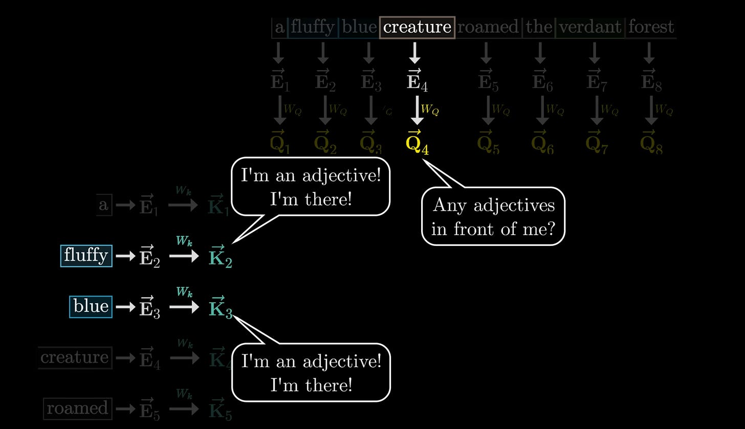
Now let’s add math. The Query (Q), Key (K), and Values (V) all represent matrices that our model can learn. This grouping represents one attention head. We take each word, and create an embedding which is a vector that we can multiply by these matrices. We do exactly as above, multiplying these matrices by our embeddings to create vectors. We can then combine these vectors to get a numeric representation as to the likelihood these words interconnect. With this numeric representation, we can then learn a final matrix, aka the Output matrix, to take these different updated representations, and make a guess at what the next word in the sequence should be.
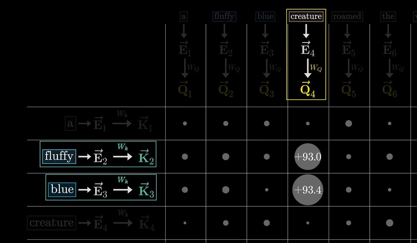
All of this is about creating numeric representations (vectors) of arbitrary data (words), and using matrix operations to combine those representations together. When we scale this up to many attention heads, each asking different questions, we are able to create a rich understanding of the data. Let’s see how this can work for our fluid LSTM.
Back to Fluids
Fluids in this case work much the same way as words did in the previous case. We have some arbitrary data (the density of fluid & the velocities of data) with which we wish to create a set of queries (how fast should I be moving, which direction, etc), a set of keys (e.g. I am your neighbor and moving fast left so should you), and use values to update the fluid for the next time step.
In the actual paper, we take the actual setup of the LSTM as described previously, and attach basically a second memory to the model using our self attention paradigm. This is called a self attention memory module (SAM).
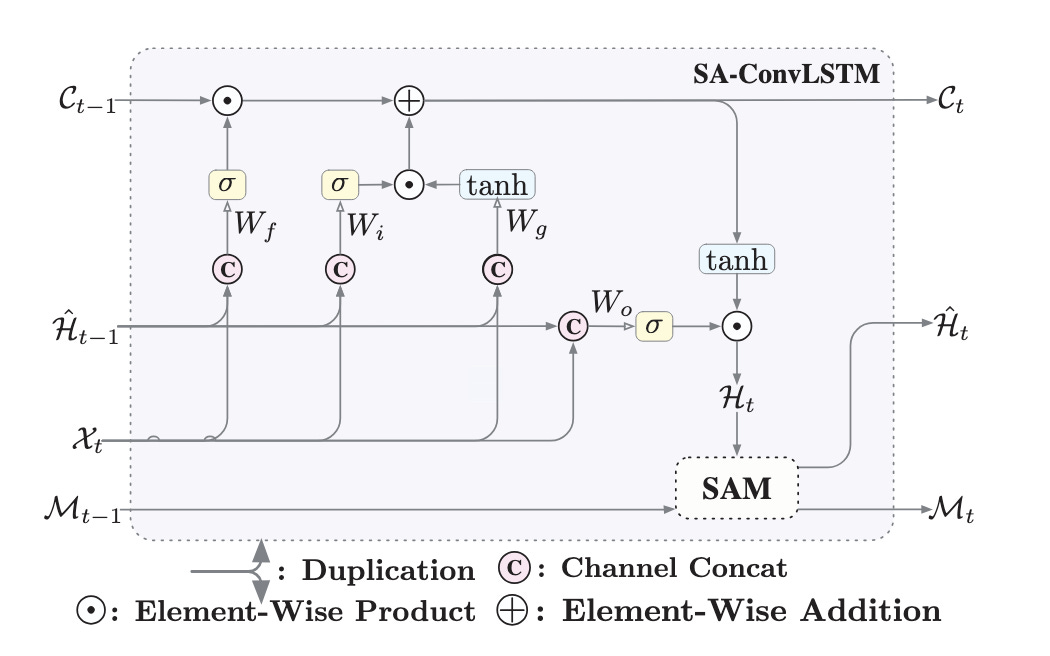
This image may look complicated, but it’s the same as the one before! We have our forget gate, input gate, and output gate affecting our long term memory, short term memory, and input. The only difference is our new SAM module with it’s own memory M also affecting the output. Our actual SAM module is exactly as described in the section on self attention, but doubled up. Once for the long term memory, and once for the Sam’s own special memory.
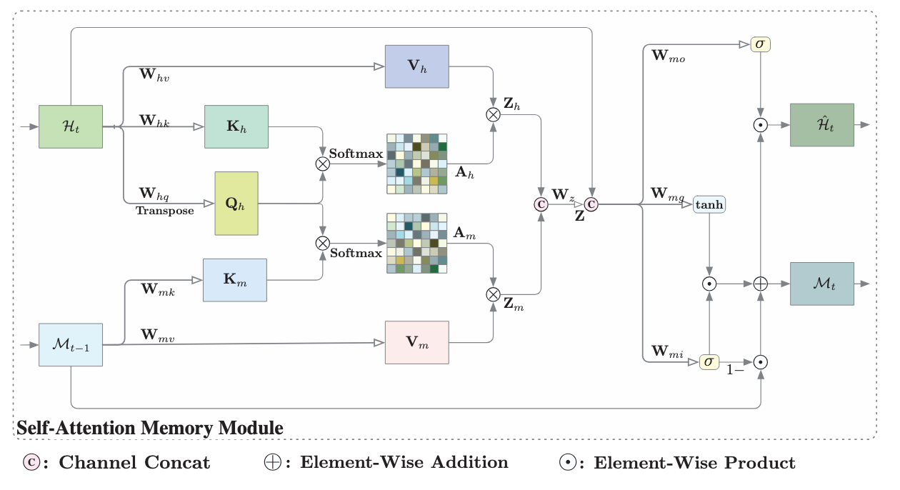
Let’s code this up.
Code
We make three major changes.
The first is to our outer loop where we initialize our memory
def forward(self, x_seq):
        ...
        memory = torch.zeros(B, self.convlstm.memory_channels, H, W, device=x_seq.device)
        ...
The second is to our inner loop, where we add the final call to the memory unit per the first image above, and return the additional new memory.
def __init__(self, input_channels, hidden_channels, memory_channels, kernel_size=3):
        ...
        self.sam = SAM(hidden_channels, memory_channels, kernel_size=kernel_size)
def forward(self, x, short_term_memory, long_term_memory, memory):
...
# Update with SAM module
short_term_memory, memory = self.sam(short_term_memory, memory)
return short_term_memory, long_term_memory, memoryThe last change is to create the actual Attention head block. We initialize the queries, keys, and values, and then multiply matrices as per the second image above. One important difference between attention in transformers and attention here is that we use convolution layers instead of just linear layers. This is the same reasoning from our convolution from the previous section, convolution is more parameter efficient and better embeds spatial data.
class SAM(nn.Module):
    def __init__(self, hidden_channels, memory_channels, kernel_size=3):
        super().__init__()
        padding = kernel_size // 2
        self.W_hq = nn.Conv2d(hidden_channels, hidden_channels, kernel_size, padding=padding)
        self.W_hk = nn.Conv2d(hidden_channels, hidden_channels, kernel_size, padding=padding)
        self.W_hv = nn.Conv2d(hidden_channels, hidden_channels, kernel_size, padding=padding)
        self.W_mq = nn.Conv2d(memory_channels, hidden_channels, kernel_size, padding=padding)
        self.W_mk = nn.Conv2d(memory_channels, hidden_channels, kernel_size, padding=padding)
        self.W_mv = nn.Conv2d(memory_channels, memory_channels, kernel_size, padding=padding)
        self.W_z = nn.Conv2d(hidden_channels + memory_channels, hidden_channels, kernel_size=1)
        self.W_mo = nn.Conv2d(memory_channels, memory_channels, kernel_size=1)

    def forward(self, H_t, M_t):
        # Compute hidden attention
        Q_h = self.W_hq(H_t)
        K_h = self.W_hk(H_t)
        V_h = self.W_hv(H_t)
        A_h = torch.softmax(torch.einsum("bchw,bcxy->bhwy", Q_h, K_h), dim=-1)
        Z_h = torch.einsum("bhwy,bcxy->bchw", A_h, V_h)

        # Compute memory attention
        Q_m = self.W_mq(M_t)
        K_m = self.W_mk(M_t)
        V_m = self.W_mv(M_t)
        A_m = torch.softmax(torch.einsum("bchw,bcxy->bhwy", Q_m, K_m), dim=-1)
        Z_m = torch.einsum("bhwy,bcxy->bchw", A_m, V_m)

        # Combine hidden and memory features
        Z = torch.cat([Z_h, Z_m], dim=1)
        H_hat_t = torch.sigmoid(self.W_z(Z))
        M_t = torch.sigmoid(self.W_mo(Z_m)) * M_t + (1 - torch.sigmoid(self.W_mo(Z_m))) * torch.tanh(Z_m)

        return H_hat_t, M_t
Which isn’t too many changes! That’s the core idea of the paper, it’s adding attention to a recurrent neural network that is very drop in. Below is the full code.
import torch
import torch.nn as nn
import torch.optim as optim
from torch.utils.data import DataLoader, Dataset

# --- SAM Module ---
class SAM(nn.Module):
    def __init__(self, hidden_channels, memory_channels, kernel_size=3):
        super().__init__()
        padding = kernel_size // 2
        self.W_hq = nn.Conv2d(hidden_channels, hidden_channels, kernel_size, padding=padding)
        self.W_hk = nn.Conv2d(hidden_channels, hidden_channels, kernel_size, padding=padding)
        self.W_hv = nn.Conv2d(hidden_channels, hidden_channels, kernel_size, padding=padding)
        self.W_mq = nn.Conv2d(memory_channels, hidden_channels, kernel_size, padding=padding)
        self.W_mk = nn.Conv2d(memory_channels, hidden_channels, kernel_size, padding=padding)
        self.W_mv = nn.Conv2d(memory_channels, memory_channels, kernel_size, padding=padding)
        self.W_z = nn.Conv2d(hidden_channels + memory_channels, hidden_channels, kernel_size=1)
        self.W_mo = nn.Conv2d(memory_channels, memory_channels, kernel_size=1)

    def forward(self, H_t, M_t):
        # Compute hidden attention
        Q_h = self.W_hq(H_t)
        K_h = self.W_hk(H_t)
        V_h = self.W_hv(H_t)
        A_h = torch.softmax(torch.einsum("bchw,bcxy->bhwy", Q_h, K_h), dim=-1)
        Z_h = torch.einsum("bhwy,bcxy->bchw", A_h, V_h)

        # Compute memory attention
        Q_m = self.W_mq(M_t)
        K_m = self.W_mk(M_t)
        V_m = self.W_mv(M_t)
        A_m = torch.softmax(torch.einsum("bchw,bcxy->bhwy", Q_m, K_m), dim=-1)
        Z_m = torch.einsum("bhwy,bcxy->bchw", A_m, V_m)

        # Combine hidden and memory features
        Z = torch.cat([Z_h, Z_m], dim=1)
        H_hat_t = torch.sigmoid(self.W_z(Z))
        M_t = torch.sigmoid(self.W_mo(Z_m)) * M_t + (1 - torch.sigmoid(self.W_mo(Z_m))) * torch.tanh(Z_m)

        return H_hat_t, M_t

# --- ConvLSTM Cell ---
class ConvLSTMCell(nn.Module):
    def __init__(self, input_channels, hidden_channels, memory_channels, kernel_size=3):
        super().__init__()
        padding = kernel_size // 2
        self.conv = nn.Conv2d(input_channels + hidden_channels, 4 * hidden_channels, kernel_size, padding=padding)
        self.hidden_channels = hidden_channels
        self.memory_channels = memory_channels
        self.sam = SAM(hidden_channels, memory_channels, kernel_size=kernel_size)

    def forward(self, x, short_term_memory, long_term_memory, memory):
        # Combine input with short-term memory (previous hidden state)
        combined = torch.cat([x, short_term_memory], dim=1)
        conv_out = self.conv(combined)

        # Split the output into gates and cell candidate
        input_gate, forget_gate, output_gate, cell_candidate = torch.chunk(conv_out, 4, dim=1)

        # Apply activations for each gate
        input_gate = torch.sigmoid(input_gate)
        forget_gate = torch.sigmoid(forget_gate)
        output_gate = torch.sigmoid(output_gate)
        cell_candidate = torch.tanh(cell_candidate)

        # Update long-term memory (cell state)
        long_term_memory = forget_gate * long_term_memory + input_gate * cell_candidate

        # Update short-term memory (hidden state)
        short_term_memory = output_gate * torch.tanh(long_term_memory)

        # Update with SAM module
        short_term_memory, memory = self.sam(short_term_memory, memory)

        return short_term_memory, long_term_memory, memory

# --- UNet + ConvLSTM Model ---
class ConvLSTMUNet(nn.Module):
    def __init__(self, input_channels=3, hidden_channels=32, memory_channels=32):
        super().__init__()

        self.encoder = nn.Sequential(
            nn.Conv2d(input_channels, 32, kernel_size=3, padding=1),
            nn.ReLU(),
            nn.Conv2d(32, 64, kernel_size=3, padding=1),
            nn.ReLU(),
        )

        self.convlstm = ConvLSTMCell(64, hidden_channels, memory_channels)

        self.decoder = nn.Sequential(
            nn.Conv2d(hidden_channels, 32, kernel_size=3, padding=1),
            nn.ReLU(),
            nn.Conv2d(32, input_channels, kernel_size=3, padding=1),
        )

    def forward(self, x_seq):
        B, T, C, H, W = x_seq.size()
        short_term_memory = torch.zeros(B, self.convlstm.hidden_channels, H, W, device=x_seq.device)
        long_term_memory = torch.zeros(B, self.convlstm.hidden_channels, H, W, device=x_seq.device)
        memory = torch.zeros(B, self.convlstm.memory_channels, H, W, device=x_seq.device)

        predictions = []
        x_t = x_seq[:, -1]
        for _ in range(100):
            x_enc = self.encoder(x_t)
            short_term_memory, long_term_memory, memory = self.convlstm(x_enc, short_term_memory, long_term_memory, memory)
            x_t = self.decoder(short_term_memory)
            predictions.append(x_t.unsqueeze(1))

        return torch.cat(predictions, dim=1)


import torch
from torch.utils.data import DataLoader

# Assuming the FluidDataset is defined as before
class FluidSequenceDataset(Dataset):
    def __init__(self, fluid_grids, history=3):
        self.history = history
        self.sequences = []
        for i in range(len(fluid_grids) - history):
            seq = []
            for j in range(history):
                g = fluid_grids[i + j]
                tensor = torch.stack([
                    torch.tensor(g.density, dtype=torch.float32),
                    torch.tensor(g.velocityx, dtype=torch.float32),
                    torch.tensor(g.velocityy, dtype=torch.float32)
                ], dim=0)
                seq.append(tensor)
            self.sequences.append(torch.stack(seq))

    def __len__(self):
        return len(self.sequences)

    def __getitem__(self, idx):
        return self.sequences[idx]

# Load data
dataset = FluidSequenceDataset(fluid_grids)
dataloader = DataLoader(dataset, batch_size=1, shuffle=False)

# Initialize the model
device = torch.device("cuda" if torch.cuda.is_available() else "cpu")
model = ConvLSTMUNet().to(device)

def train_model(model, dataloader, epochs=50, lr=0.001):
    optimizer = optim.Adam(model.parameters(), lr=lr)

    for epoch in range(epochs):
        total_loss = 0.0
        for seq_batch in dataloader:
            seq_batch = seq_batch.to(device)
            target = seq_batch[:, -1]  # supervise with next step

            optimizer.zero_grad()
            prediction = model(seq_batch)[:, 0]  # only predict one step for training

            # Base loss (reconstruction)
            loss = nn.functional.mse_loss(prediction, target)

            loss.backward()
            optimizer.step()
            total_loss += loss.item()

        print(f"Epoch {epoch+1}/{epochs}, Loss: {total_loss/len(dataloader):.6f}")


train_model(model, dataloader)

# Set the model to evaluation mode
model.eval()

# Predict 100 future timestamps and store in new array
with torch.no_grad():
    sample_seq = dataset[0].unsqueeze(0).to(device)  # (1, T, C, H, W)
    future_predictions = model(sample_seq)  # (1, 100, C, H, W)
    print("Future prediction shape:", future_predictions.shape)

    # Extract density channel (index 0)
    future_densities = future_predictions[:, :, 0, :, :]  # (1, 100, H, W)
    print("Future density shape:", future_densities.shape)


# Predict 100 future timestamps
future_densities_arr = future_densities.squeeze(0).cpu().numpy()

for i, frame in enumerate(future_densities_arr):
  save_density_frame(frame, i)

create_gif()

gif_path = "fluid_sim.gif"  # Replace with the actual path if needed

# Display the gif
Image(filename=gif_path)
And there is the results
😔
I’m not really sure why this was worse? I guess the attention head perhaps needs more data to make something usable? Or maybe my training is wrong someway between this and the convolution code but I don’t see anything.
Conclusion
There is an old saying in machine learning: “Changing one thing changes everything”. Changing the model may change your data requirements may change your training loop may change everythinge else. While Recurrent Neural Networks are a step in the right direction, we still have a ways before we can really do anything with it.
Work Cited
Original LSTM Paper by Hochreiter and Schmidhuber
ConvLSTM by Shi et al
Self-Attention ConvLSTM by Lin et al

